What I learned predicting churn with XGBoost

I started with a fairly simple question: could I identify customers who were more likely to leave, early enough for someone to do something useful with that information? I built the model in Python, using XGBoost inside a scikit-learn pipeline. Getting a prediction out was the straightforward part. Working out how much I could trust it took considerably more thought.

The label came before the model

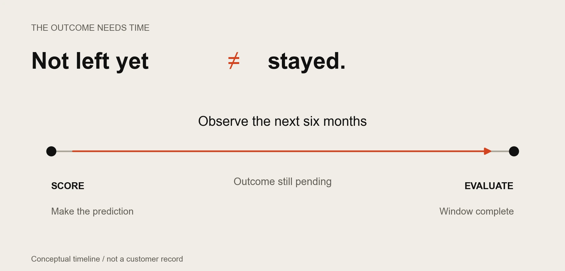
I defined churn over a six-month window. That sounds tidy, until you realise that a recent customer who has not left yet is not necessarily a non-churner. They may simply not have had enough time to leave. I excluded records without a complete outcome window from training and evaluation. Otherwise, I would have been teaching the model that “we do not know yet” meant “stayed”.

XGBoost was a practical choice

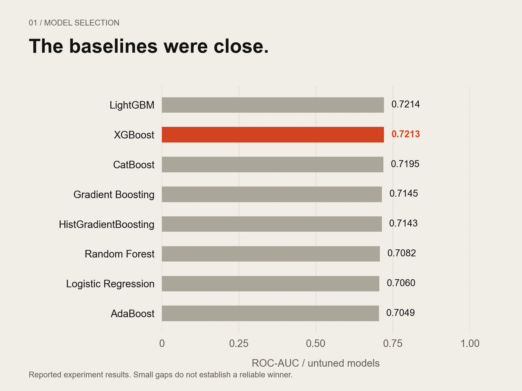
I compared eight algorithms before tuning. The boosted tree models were close: LightGBM edged XGBoost on ROC-AUC, while XGBoost edged LightGBM on PR-AUC. Those tiny differences did not give me a convincing outright winner. I chose XGBoost for the wider combination of useful ranking, class weighting, explainability and manageable deployment.

I kept preprocessing and inference in one pipeline, so missing values and categorical inputs were handled consistently. For tuning, I used successive halving to explore broadly, then a smaller grid search around promising settings. MLflow helped me keep track of the runs. It was a more manageable process than letting a huge grid search run overnight and trying to reconstruct what had changed afterwards.

A useful score needs a decision around it

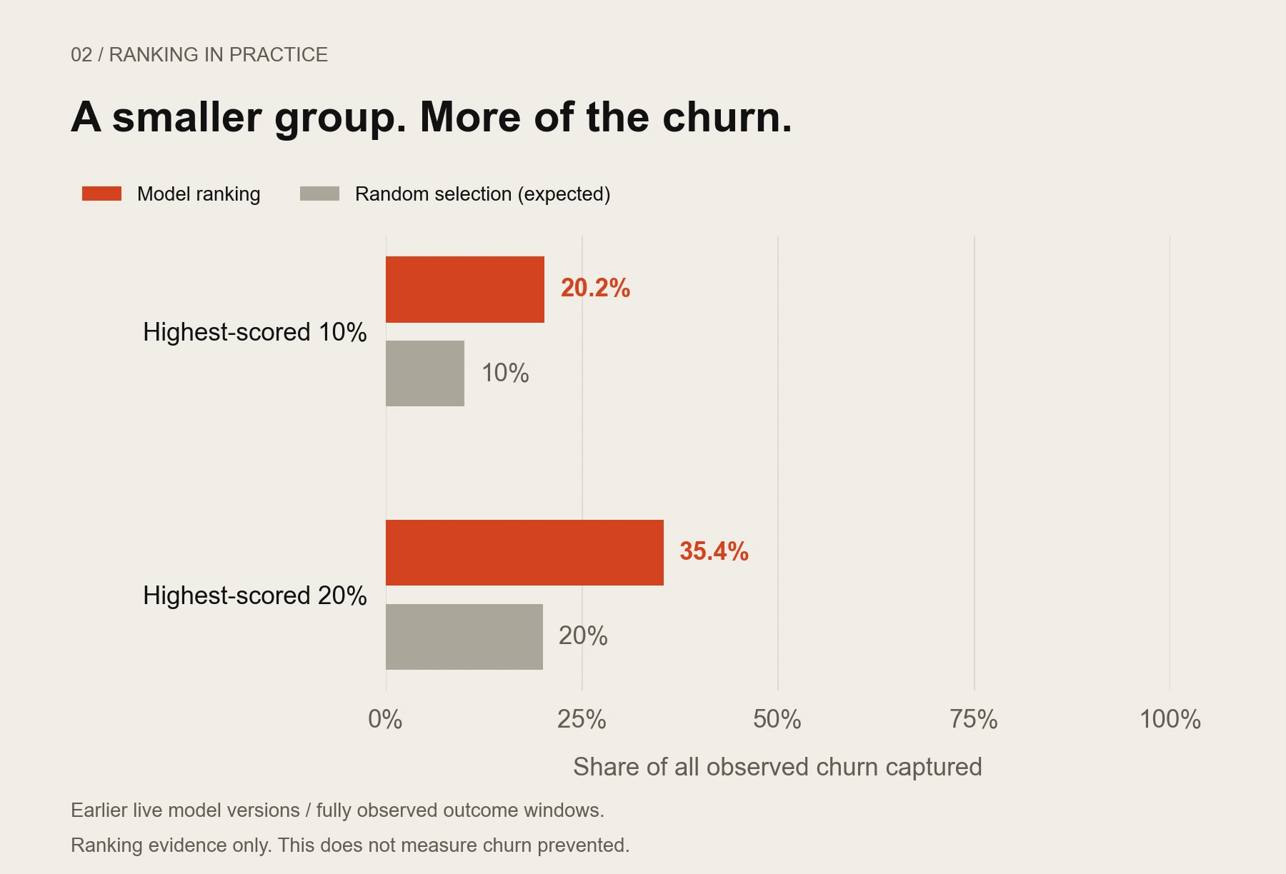
Churn was the minority class. A model could look reassuringly accurate while missing the people I wanted to find, so I paid closer attention to recall, precision and ranking. Class weighting helped make missed churners more costly during training. It also meant I could not safely read the raw scores as calibrated probabilities: a score of 0.7 was not evidence that exactly 70% of similar customers would leave.

Choosing a threshold was a separate decision. Catching more churners meant flagging more people who would stay, and creating more work for whoever reviewed the predictions. Changing that boundary changed the labels and workload; it did not change the underlying scores. I also learned to freeze thresholds before evaluating on fresh outcomes. Revisiting boundaries using the same evaluation data can make the results look better than they really are.

Explanations needed translating

SHAP helped me inspect what pushed an individual prediction up or down. But an encoded column name and a contribution value were not particularly useful to someone reviewing a customer. Translating them into plain labels and recognisable values became part of the work. I treated those explanations as clues about the model’s reasoning, not proof of why somebody would leave.

I also tested removing demographic and geographic inputs. Validation performance barely moved, which gave me a good reason to leave them out. That was a useful finding in its own right: a longer feature list was not automatically a better one. Removing those fields did not prove the model was fair, though; other inputs can still carry related patterns, so group-level checks remained necessary.

The notebook was only the beginning

The later model achieved about 0.731 ROC-AUC on a chronological hold-out. Earlier live versions recorded about 0.649 once their outcomes had matured. I could not treat that gap as a measured decline in the same model: the versions, cohorts and periods were different. It was a reason to investigate and keep collecting evidence.

The six-month target also meant waiting six months to evaluate each new prediction properly. In the meantime, I checked inputs, missingness, batch completion and score distributions. A distribution shift could prompt an investigation, but could not tell me on its own whether predictions had become worse. Calibration and evaluation on fresh, fully observed cohorts are the next improvements I want to make.

The biggest change in my thinking was learning to judge the whole process around the score: what the label means, what was known at prediction time, how someone uses the result, and when the evidence is actually ready. XGBoost gave me a useful model. Those questions taught me how to evaluate it more honestly.